Millions of records, one Spark job.
The catalog covers seismic events recorded between January 1970 and March 2019: coordinates, depth, magnitude and its scale, station counts and recording-quality measures. At this size, pandas on one core is not the right tool, so everything runs on Spark DataFrames and MLlib, in parallel across all local cores.
| Stage | Records | What happens |
|---|---|---|
| Original catalog | 3,272,774 | 23 columns, earthquakes and other seismic events |
| After deduplication | 3,256,955 | duplicate rows removed |
| Clean earthquake catalog | 2,607,588 | earthquakes only, 13 columns, no missing values |
| After outlier filtering | 2,607,556 | 32 extreme points removed after PCA |
The four stages the demo at the top animates, with the record counts saved in the notebooks.
Recover the data, do not drop it.
Four informative columns had large holes. Dropping them, or dropping every row with a gap, would have thrown away most of what the catalog says about how each event was recorded:
So I imputed them, each with the simplest method that fits: the mean for dmin and gap, a linear regression for nst and a decision-tree regression for magNst, both trained on latitude, longitude, depth, magnitude and RMS residual. Observed values were never touched; only the missing ones received a prediction. At the end, no column has a single null left.
# 'nst' is imputed by linear regression on five columns that are always presentcolumns_to_use = ['latitude', 'longitude', 'depth', 'mag', 'rms']assembler = VectorAssembler(inputCols=columns_to_use, outputCol="features")scaler = StandardScaler(inputCol="features", outputCol="scaledFeatures")lr = LinearRegression(featuresCol="scaledFeatures", labelCol='nst')pipeline = Pipeline(stages=[assembler, scaler, lr])# train on the rows where 'nst' is known, then predict for every rowmodel = pipeline.fit(df.filter(df.nst.isNotNull()))full_predictions = model.transform(df)# observed values are kept; only the missing ones take the predictiondf_imputed = full_predictions.withColumn( "nst_imputed", when(full_predictions["nst"].isNull(), full_predictions["prediction"]) .otherwise(full_predictions["nst"]))Eight kinds of earthquake.
I clustered the catalog with Spark's K-Means (k-means|| initialization) on nine standardized features: position, depth, magnitude, station counts, azimuthal gap, nearest-station distance and RMS residual. SSE and silhouette curves guided the choice of eight groups. A PCA projection, applied after clustering to look at the result, exposed 32 extreme points, which I filtered out.
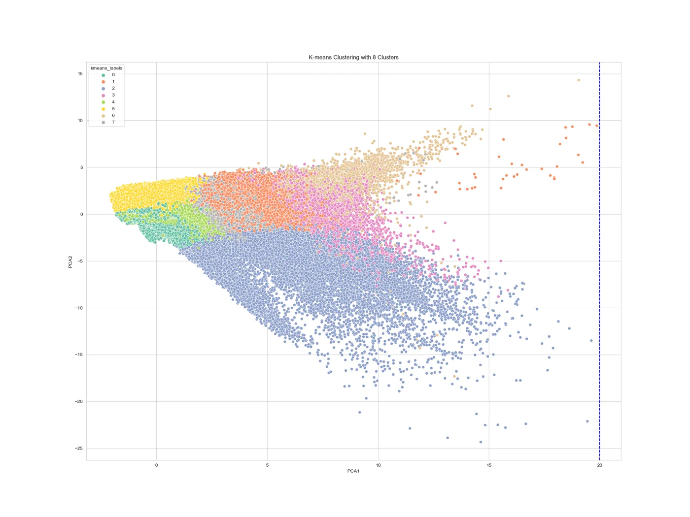
The cluster statistics read like a seismology summary:
| Group | Events | Depth (km) | Magnitude | Stations | Gap (°) | dmin |
|---|---|---|---|---|---|---|
| 0 shallow, small | 1,228,039 | 6.08 | 1.31 | 15.60 | 90.95 | 0.09 |
| 1 | 199,238 | 57.69 | 4.52 | 39.21 | 121.43 | 0.83 |
| 2 well recorded | 38,944 | 39.88 | 4.21 | 131.69 | 68.64 | 0.65 |
| 3 deep | 25,368 | 498.41 | 4.44 | 56.31 | 118.63 | 1.41 |
| 4 | 469,400 | 35.33 | 1.68 | 24.17 | 124.57 | 0.31 |
| 5 poor coverage | 472,058 | 8.51 | 1.30 | 7.71 | 217.02 | 0.18 |
| 6 remote | 4,612 | 36.49 | 4.62 | 42.97 | 116.95 | 20.91 |
| 7 | 169,897 | 33.48 | 3.91 | 41.46 | 125.10 | 0.48 |
Means per group. Group 3 gathers the deep earthquakes, from 242 down to 735.8 km; group 6 the events far from any station; group 2 the best-recorded ones.
The same catalog, by geography.
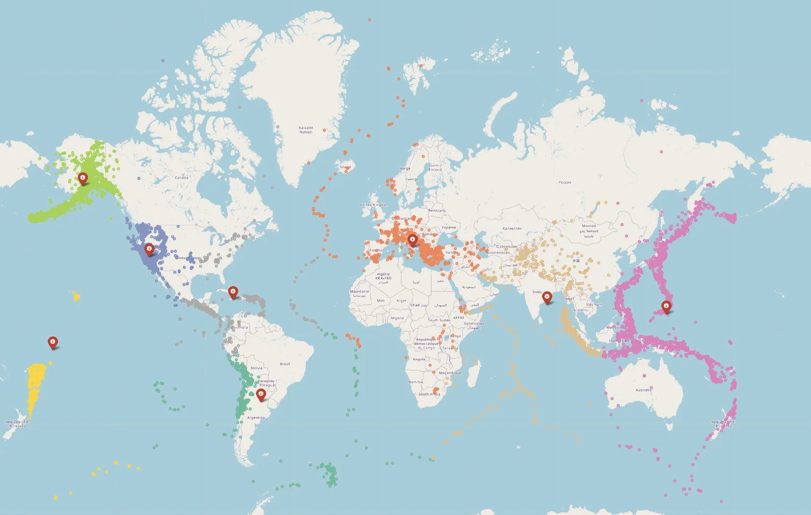
A second K-Means, on latitude and longitude only, organized the events into eight geographical areas, then Folium turned them into interactive world maps. The largest area holds 1,655,188 events, 63.48% of the catalog, in the western United States: that is where the densest station networks are. The others separate Alaska, the western Pacific, Europe, South America and New Zealand.
Strong events, and the threshold that finds them.
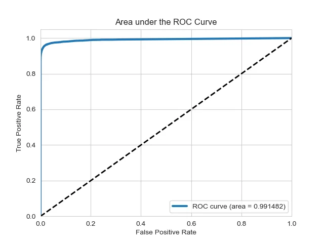
The last notebook classifies each recorded event as magnitude 3 or above (17.61% of the catalog) or below 3, from a 19-feature vector, with an 80/20 split, four-fold cross-validation and ROC AUC as the metric:
With only 17.6% of positives, accuracy hides what matters: how many strong events the model misses. Lowering the forest's decision threshold from the default to 0.3 changes the trade-off:
| Threshold | Missed strong events | False alarms | Recall, strong events |
|---|---|---|---|
| Default | 7,425 | 1,183 | 91.89% |
| 0.3 | 5,368 | 3,458 | 94.14% |
The lower threshold misses 27.7% fewer strong events at the cost of more false alarms. Which side to favor is a decision about the cost of each error, and the analysis puts both numbers on the table.
Four notebooks, one catalog.
The report and the notebooks document every step, from the first schema inspection to the threshold analysis, with the interactive Folium maps.