21,909 titles, prepared with care.
The dataset combines release dates, runtime, votes, reviews, awards, credits, title types, genres and countries for 21,909 titles, split into 16,431 for training and 5,478 for testing. Every preparation step was fitted on the training data only and then applied to the test data:
- Missing values. Runtime placeholders became missing values imputed with the training median; missing award counts were estimated with IterativeImputer.
- Categories. Ordinal encoding for ratings, one-hot for title types, indicators for the ten most frequent genres and countries.
- Redundancy and skew. Pearson, Spearman and Cramér's V guided which attributes to drop; skewed counts went through log1p and standardization.
- Outliers. Local Outlier Factor (20 neighbors, 5% contamination) removed 822 training rows, leaving 15,609 titles.
Three algorithms, three stories.
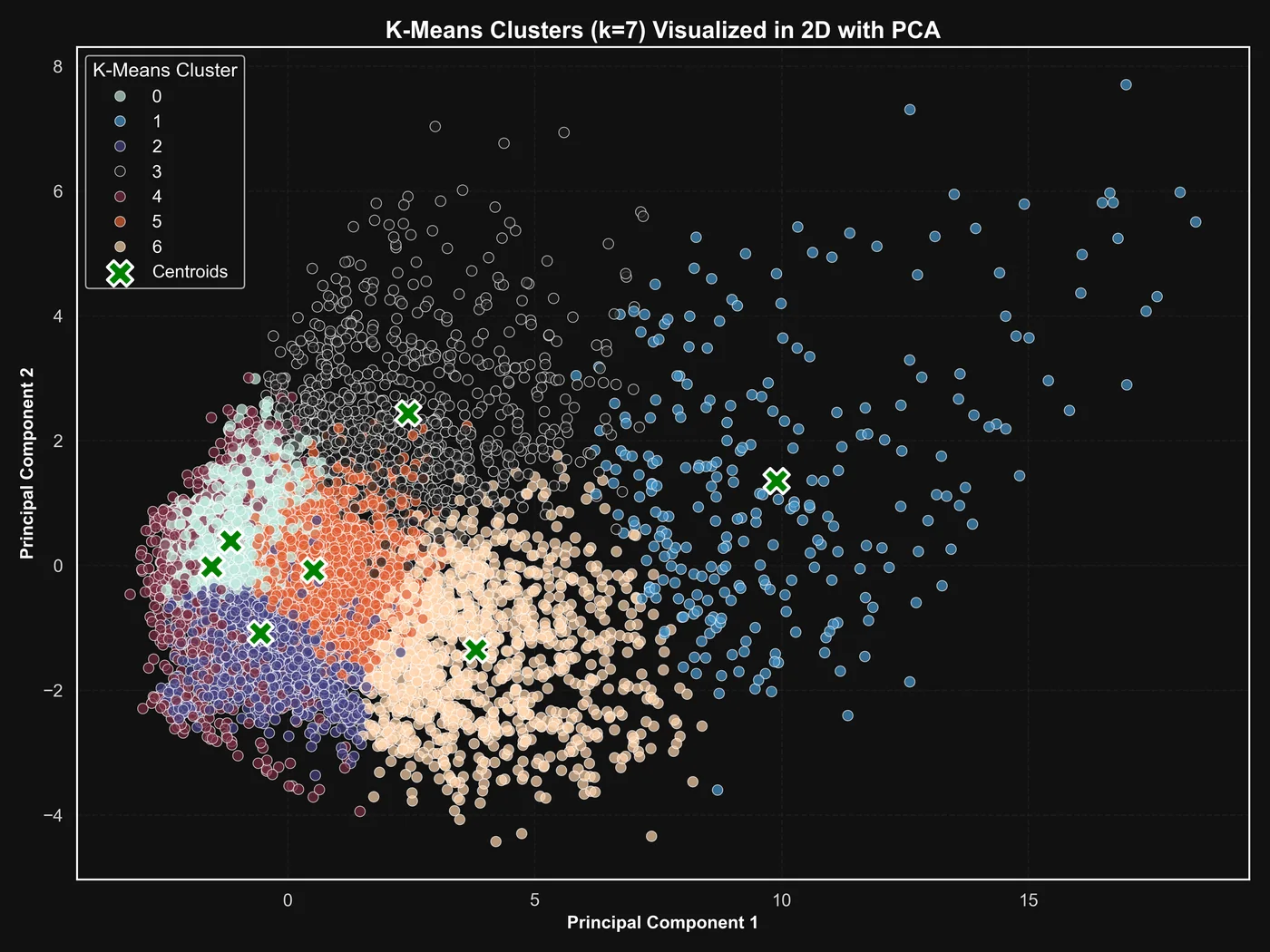
I clustered the same 11 numerical features with three methods and read every group through its original metadata: genres, title types, countries and representative titles.
| Method | How it was tuned | What it found |
|---|---|---|
| K-Means | inertia and silhouette for k = 2 to 50, plus domain reading | 7 segments: mainstream hits, award-oriented titles, vintage cinema, shorts, television, low visibility |
| DBSCAN | k-distance curve, ε = 1.5, min 12 samples | 3 clusters + noise, with 1,884 titles labeled noise |
| Hierarchical | single, complete, average and Ward linkage compared on dendrograms | 5 Ward groups: acclaimed, popular, vintage, television, low engagement |
Predicting the rating tier.
Ratings were grouped into three tiers, Poor (up to 6.0), Average (6.0 to 7.0) and Good (above 7.0), and predicted from 41 features. Every model was tuned with cross-validation and evaluated on the 5,478 test titles:
The middle tier, Average, was the hardest to separate for every model, which confusion matrices, per-class metrics and ROC curves make visible. The decision tree adds a readable view of what matters: title type, release year, genre and popularity.
From patterns to predictions.
Each title became a transaction of 61 Boolean items, from discretized numbers to genres, plus the target: at least one award win. FP-Growth with 3% minimum support produced 75 rules whose consequent is an award. One of the strongest:
Among titles matching this combination, 57.1% have won an award, against about 13.1% overall. I then turned the rules into a custom rule-based classifier: a title is predicted as a winner when a qualifying rule matches it, and a confidence threshold controls how selective the rules are.
| Minimum rule confidence | Precision | Recall | F1 |
|---|---|---|---|
| 25%: broad screening | 17.95% | 81.11% | 0.29 |
| 50%: selective | 40.36% | 39.53% | 0.40 |
Award-winner class on the test set. The screening setting finds 554 of the 683 winners; the selective one more than doubles precision.
class RuleBasedClassifierV2: """ Version 2 of the classifier: a confidence threshold makes the model more selective. """ def __init__(self, rules, confidence_threshold=0.0): self.rules = rules.copy() self.rules['antecedents'] = self.rules['antecedents'].apply(lambda x: frozenset(x)) self.confidence_threshold = confidence_threshold def predict(self, X_trans): """ Predicts on a transactional DataFrame. """ predictions = [] for i, row in X_trans.iterrows(): transaction_items = set(row[row].index) prediction = False for _, rule in self.rules.iterrows(): # a rule fires only if it matches the title and its confidence is high enough if rule['antecedents'].issubset(transaction_items) and rule['confidence'] >= self.confidence_threshold: prediction = True break predictions.append(prediction) return pd.Series(predictions, index=X_trans.index)Predicting audience engagement.
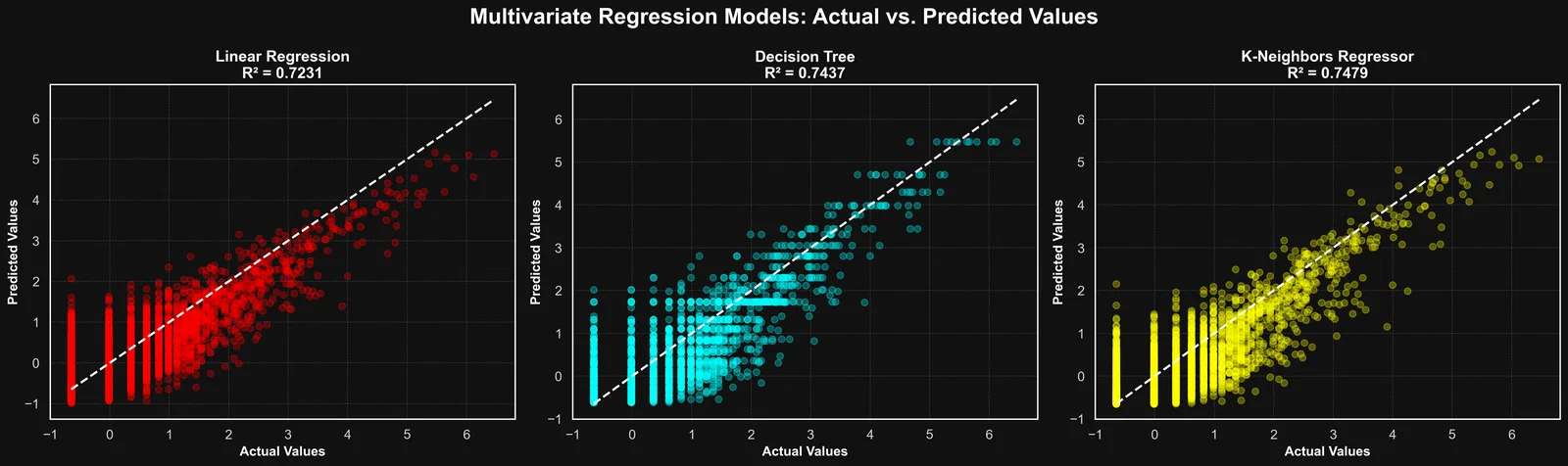
The last task predicts the number of user reviews (log-transformed and standardized) from one predictor, the vote count, and then from six: votes, critic reviews, regions, award nominations, credits and award wins.
| Regressor | R², 1 predictor | R², 6 predictors | MAE | RMSE |
|---|---|---|---|---|
| Linear Regression | 0.6402 | 0.7231 | 0.3883 | 0.5247 |
| Decision Tree | 0.6893 | 0.7437 | 0.3636 | 0.5049 |
| K-Nearest Neighbors | 0.6846 | 0.7479 | 0.3628 | 0.5007 |
Five stages, one workflow.
The report and the nine notebooks document every step, from data understanding to the rule-based classifier and the regression comparison.