SoundPulse — Explainable Machine Learning on Spotify

114 genres, ten families.

The public Spotify catalog has 114,000 tracks, 1,000 for each of 114 genres. Every track comes with metadata (artists, album, popularity, explicit flag) and Spotify's audio descriptors: danceability, energy, loudness, speechiness, acousticness, instrumentalness, liveness, valence, tempo, key, mode and duration.

Many of those genres overlap, so I designed a taxonomy by hand that folds the 114 genres into 10 macro-genres: metal, black-metal, death-metal, grindcore and metalcore become Metal & Hardcore; k-pop, j-pop, anime, cantopop, afrobeat and reggae become World & Regional. I also merged key and mode into one readable feature, such as "C# minor", with 24 values.

The result is realistically imbalanced, a deliberate challenge for every classifier that follows. Exploration also gave the first hint about popularity: it has almost no monotonic correlation with any single audio feature (|ρ| ≤ 0.08), while energy goes with loudness (ρ = 0.75) and against acousticness (ρ = −0.71). Whatever drives popularity, it is not one feature on its own.

The 5% that do not fit.

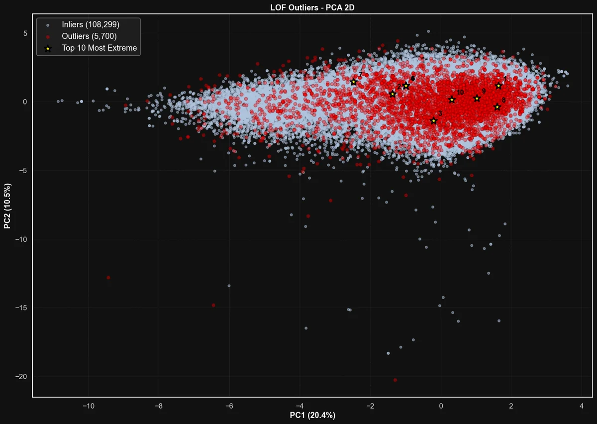
Tracks were screened in a 47-dimensional space: 13 standardized numerical features plus one-hot key and macro-genre. The number of neighbors was not guessed: the knee of the k-distance curve set k = 15. With a 5% contamination, Local Outlier Factor flagged 5,700 tracks, the same method the demo at the top runs on toy data.

The most extreme ones are easy to explain: tracks with zero popularity surrounded by very popular look-alikes, such as songs by Kid Cudi and Wiz Khalifa on compilation albums, and exact duplicates of one song listed under three genres (folk, songwriter and singer-songwriter), a classic data-quality issue.

Nine sound families, and proof they are real.

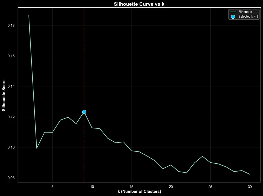
I ran K-Means (k-means++ initialization, Elkan algorithm) for k from 2 to 50, and computed the silhouette for k from 2 to 30 on a 20,000-track sample, detecting its local maxima automatically. k = 9 was the best non-trivial peak (silhouette 0.123), in agreement with the elbow of the inertia curve.

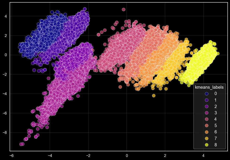
Clusters can be artifacts of the algorithm. If a supervised model can recover them from the raw features, they are not. I trained two validators to predict the cluster label:

The tree also says what defines the segments: energy, instrumentalness, explicit content, popularity and danceability. That gives every cluster a direct business reading, such as "high-energy explicit tracks" against "quiet instrumental tracks".

Ten genres from 13 numbers.

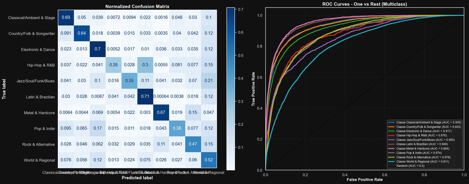
The central task: predict one of the 10 macro-genres from only 13 standardized audio and metadata features, with a stratified 70/30 split (75,809 training and 32,490 test tracks). I built two very different models.

A tuned Random Forest

A grid search over 160 configurations with five-fold stratified cross-validation (800 fits), optimizing macro F1 with balanced class weights.

A residual deep network, designed from scratch

For tabular, imbalanced, multi-class data: 4,649,034 parameters, residual blocks with LayerNorm and GELU, an attention-style sigmoid gate, decaying dropout from 0.45 to 0.10, AdamW with a 10-epoch warm-up and cosine annealing, and class weights smoothed with a 0.75 power so that rare genres count without dominating. Trained on an Apple M3 Ultra GPU through TensorFlow-Metal, best checkpoint at epoch 197.

input_layer = layers.Input(shape=(X_train.shape[1],))# Block 1: initial feature extractionx = layers.Dense(1536, kernel_initializer=he_init, kernel_regularizer=l2_reg)(input_layer)x = layers.LayerNormalization()(x)x = layers.Activation('gelu')(x)x = layers.GaussianNoise(0.1)(x, training=True)x = layers.Dropout(0.45)(x)# Block 2: deep feature learning with a skip connectionx_res = layers.Dense(768, kernel_initializer=he_init)(x)x = layers.Dense(768, kernel_initializer=he_init, kernel_regularizer=l2_reg)(x)x = layers.LayerNormalization()(x)x = layers.Activation('gelu')(x)x = layers.Dropout(0.4)(x)x = layers.Dense(768, kernel_initializer=he_init, kernel_regularizer=l2_reg)(x)x = layers.LayerNormalization()(x)x = layers.Add()([x, x_res])  # residual connectionx = layers.Activation('gelu')(x)x = layers.Dropout(0.35)(x)

Genre boundaries are fuzzy (indie-pop or synth-pop? latin or reggaeton?), so for a playlist-tagging assistant the right genre among the top three suggestions 84% of the time is the number that matters. The network also knows when it is unsure: its mean confidence is 0.74 on correct predictions and 0.55 on wrong ones.

Opening both black boxes.

• The network, with permutation importance (five repeats): popularity, energy, danceability, acousticness and loudness lead, and the top eight features explain 80% of its decisions.
• The network, with gradients per genre (∂p(genre)/∂x through tf.GradientTape): Electronic & Dance reacts to danceability, loudness and duration; Country & Folk reacts most to speechiness.
• The forest, with SHAP (TreeExplainer, a 500 × 13 × 10 tensor of values): acousticness is the strongest separator overall and the top feature for 5 of the 10 genres.

SHAP also explains single predictions. For an Electronic & Dance track the forest classified correctly, low acousticness and high danceability do most of the work:

Redrawn from the SHAP waterfall in the notebook. The same analysis is run on a misclassified Hip-Hop track, to see where the model goes wrong.

Popularity lives in the interactions.

Predicting the popularity score from 12 audio features, with every non-linear model tuned by repeated K-fold (5 folds × 2 repeats) on R², RMSE and MAE:

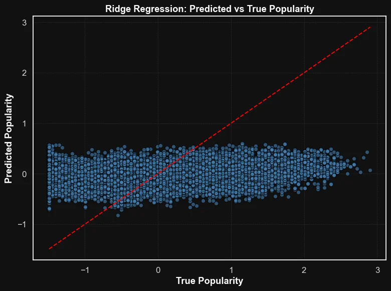
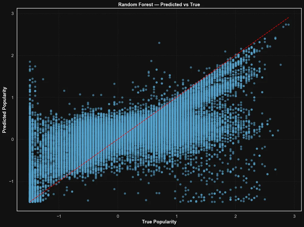
From linear models to ensembles, R² grows about 18 times, from 0.029 to 0.529, and the forest's out-of-bag R² of 0.531 confirms it. No single feature explains popularity, but their interactions explain more than half of it. The strongest drivers are valence, acousticness, duration, instrumentalness and danceability.

Catching the 9%.

The last task flags explicit lyrics: 99,181 clean tracks against 9,118 explicit ones. A model that always answers "clean" is 91% accurate, so every pipeline was tuned and compared on macro F1, recall on explicit tracks and ROC AUC, with resampling inside an imblearn pipeline:

SMOTE raised recall on explicit tracks from 39.5% to 62.8%, +59% relative, and macro F1 from 0.760 to 0.795, for a ROC AUC only 0.4 points lower. The right choice depends on the cost of each error: SMOTE is the best general trade-off, Tomek links with undersampling suit a parental-control filter that must miss almost nothing (87% recall), and the plain model suits cases where false alarms must stay rare.

# SMOTE inside the pipeline: synthetic tracks are created in the training folds onlypipeline = Pipeline(steps=[    ("smote", SMOTE(random_state=42)),    ("rf", RandomForestClassifier(random_state=42, n_jobs=-1))])param_grid = {    "rf__n_estimators": [300],    "rf__max_depth": [20, 30, None],    "rf__min_samples_split": [2, 3],    "rf__min_samples_leaf": [1, 2],    "rf__max_features": ["sqrt"],    "rf__criterion": ["entropy"]}cv = StratifiedKFold(n_splits=5, shuffle=True, random_state=42)grid_search_smote = GridSearchCV(estimator=pipeline, param_grid=param_grid,                                 scoring="f1_macro", cv=cv, n_jobs=-1, refit=True)grid_search_smote.fit(X_train, y_train)