Two datasets, one investigation.
The project asks three questions. What predicts how a title is rated? What does a model actually use to decide? And can the shape of a film's daily revenue reveal its commercial lifecycle? To answer them it works on two kinds of data: the IMDb metadata of almost 150,000 titles, and the first 100 days of box-office revenue of 1,134 films.
Preparation came first: duplicates and redundant attributes removed with Pearson, Spearman and Cramér's V, IMDb placeholders and list-like fields parsed, and missing runtimes estimated with IterativeImputer. I engineered five features from domain knowledge:
| Feature | What it captures |
|---|---|
| winRate | Award wins relative to wins plus nominations |
| contentRichness | Quotes, videos, images and credits: how complete an entry is |
| logPopularityScore | Votes times review volume, on a log scale |
| criticUserRatio | Critic reviews relative to user reviews |
| hasWriterAndDirector | Whether both credits are available |
Vote counts and credits span several orders of magnitude, so every numerical feature went through a three-stage pipeline: RobustScaler → Yeo-Johnson → StandardScaler. The original values were kept alongside, to read the results in real units later.
Three detectors, one vote.
Each anomaly detector has its own idea of "unusual": Isolation Forest looks for points that are easy to isolate, LOF for points less dense than their neighbors, CBLOF for points far from any cluster. Each one flagged about 1% of the data. A title was removed only when at least two of them agreed.
The consensus selected 1,089 titles, 0.73% of the data. They are not data errors: they are hugely popular, long-running series such as Sons of Anarchy, Family Guy and Scrubs, with up to 369,380 votes against a dataset mean of about 1,085. Removing them keeps the models focused on typical titles.
# consensus: a title counts as an outlier only if at least two of the three detectors agreedata['outlier_agreement'] = (data['outlier_isolation_forest'] + data['outlier_lof'] + data['outlier_cblof'])data['is_outlier_final'] = (data['outlier_agreement'] >= 2).astype(int)outliers_to_remove_mask = data['outlier_agreement'] >= 2data_cleaned = data[~outliers_to_remove_mask].copy()Finding the 4%.
To study learning on rare classes, I built a documentary detector on a deliberately skewed dataset: 96% other titles, 4% documentaries. A model that never predicts "documentary" is already 96% accurate, so accuracy is useless here. I kept the same Decision Tree and changed only the training data: original, oversampled with SMOTE, or randomly undersampled, always resampling the training split only.
The baseline finds fewer than one documentary in five. Both resampling strategies lift recall to almost 90%, and SMOTE gives the best F1. The precision-recall curves make the price explicit: more documentaries found also means more false alarms, a trade-off to choose with the business, not by default.
Ten rating classes, explained.
The hardest task keeps all ten IMDb rating intervals, from (0, 1] to (9, 10], with rare extreme classes and neighbors that blur into each other. I compared linear models, tree ensembles and a weighted softmax neural network (256-128-64 units with batch normalization, Gaussian noise, L2 and dropout), tuned with cross-validation:
Tree ensembles more than doubled the score of the linear models. The weighted network stopped ignoring the rare classes but paid in precision: the analysis points to the noise in human ratings, more than model capacity, as the real ceiling.
Then I opened the best model with SHAP, on three levels: global importance per class, waterfall plots for single titles, and decision plots that compare how contributions add up across titles.
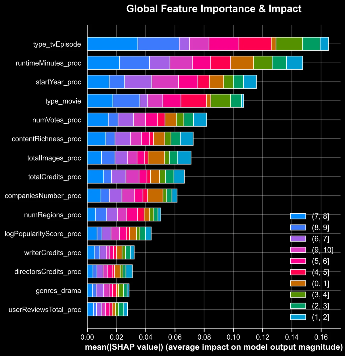
- Content type comes first. TV episodes show stable, predictable rating patterns, and the model leans on that.
- Runtime is not linear. Very short and very long titles go with lower ratings, moderate lengths with higher ones.
- Newer productions score higher, and engagement (votes) and content richness act as proxies for quality.
Predicting the rating itself.
Treating the rating as a continuous number from 1 to 10, I compared bagging and boosting, tuned with five-fold cross-validation on RMSE:
| Model | MAE | RMSE | R² |
|---|---|---|---|
| AdaBoost | 0.6115 | 0.8825 | 0.5682 |
| Random Forest | 0.6230 | 0.8921 | 0.5588 |
Errors in rating points on the original scale. The Random Forest's out-of-bag R² of 0.5632 sits right next to its test R², an independent check that the estimate is stable.
Five ways a film earns its money.
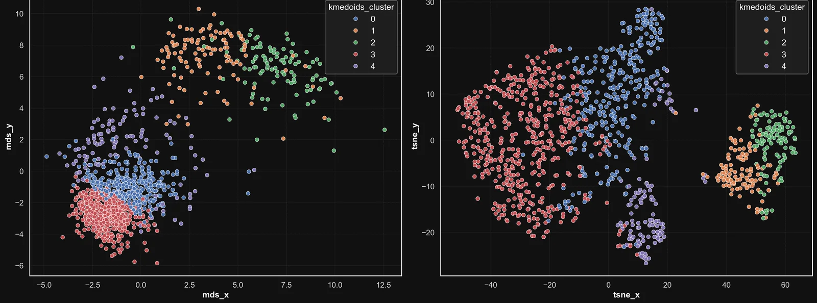
To compare revenue curves by shape rather than size, each film was z-normalized on its own. Dynamic Time Warping then measured how similar two curves are while allowing them to stretch in time, as in the demo at the top. On the 1,134 × 1,134 distance matrix I ran K-Medoids (PAM): unlike K-Means, its centers are real films, which makes every group easy to read.
The silhouette, computed for k from 2 to 20, peaked at k = 2: statistically clean, but too coarse to say anything useful. I chose k = 5 for interpretable detail. Hierarchical clustering with average linkage, tried as a comparison, collapsed into one macro-cluster with over 80% of the films, so I set it aside.
Front-loaded blockbuster
Peak in the first days, then fast decay. Action, adventure and sci-fi, rated high or medium-high.
High-variance performer
No clear trend, irregular peaks. Horror, thriller and niche sci-fi with polarized fans.
Sustained success
Strong opening and a long plateau. Animation, adventure and comedy, rated high.
Long-tail performer
Modest peak, slow steady decline: the market's baseline. Drama, comedy and romance.
Slow-burn niche success
Quiet start, late peak: the sleeper hit. Documentary, music and biography.
films in five groups, K-Medoids on DTW distances. The curves are schematic, drawn from the report's description of each medoid.
# DTW distances between the 1,134 per-film z-normalized revenue curvesdist_matrix_dtw = cdist_dtw(ts_zscore, n_jobs=-1)# K-Medoids (PAM) on the precomputed matrix: silhouette for k = 2 ... 20for k in range(2, 21): kmedoids = KMedoids(n_clusters=k, metric='precomputed', method='pam', init='k-medoids++', random_state=42) labels = kmedoids.fit_predict(dist_matrix_dtw) score = silhouette_score(dist_matrix_dtw, labels, metric='precomputed')# k = 5, keeping the best of ten initializationsOPTIMAL_K = 5for i in range(10): kmedoids_ = KMedoids(n_clusters=OPTIMAL_K, init='k-medoids++', metric='precomputed', method='pam', random_state=42 + i) labels = kmedoids_.fit_predict(dist_matrix_dtw) score = silhouette_score(dist_matrix_dtw, labels, metric='precomputed') if score > best_score: best_score = score kmedoids = kmedoids_Motifs, discords and four classifiers.
A matrix profile (STUMPY) searched all the curves for recurring 15-day patterns. The most frequent one, a sharp early peak followed by a gradual decline, appears in two Action/Drama films both rated 7.3. The most unusual one, the discord, is a late, anomalous rise in a sci-fi film rated 8.3. A shapelet model trained to recognize Action/Drama films learned the same early-peak shape on its own.
Finally, I predicted a film's rating category (four classes, 1,124 films, 899 for training and 225 for testing) from its revenue curve alone, with four different families of classifiers:
MiniROCKET won on both metrics and trained in about half a second. The surprise was DTW: here it did worse than plain Euclidean distance and was over 2,000 times slower. Box-office curves turned out to differ more in shape and amplitude than in timing, which is exactly what the comparison was there to find out.
Nine notebooks, one story.
Every step, table and figure behind this page, from the first statistics to the last classifier, is in the report and the notebooks.