Sparse regression with a hard budget.
Lasso regression fits a linear model while keeping only the features that matter: its ℓ₁ constraint pushes the weights of irrelevant features to exactly zero. In the constrained form, the budget t is a hard limit on the total size of the coefficients, so the model can be controlled directly.
Two things make it harder than it looks. The ℓ₁ norm is not differentiable, so plain gradient methods do not apply. And general-purpose solvers such as OSQP and SCS see it as just another quadratic program, ignoring the structure that could make it fast.
Remove the kink, keep the structure.
Writing every coefficient as the difference of two non-negative parts, , turns the ℓ₁ norm into a linear function. The problem becomes an equivalent convex quadratic program with linear constraints only:
From its Lagrangian I derived the dual problem and the KKT conditions. An interior-point method relaxes their complementarity conditions with a barrier parameter and follows the central path, the curve of solutions of the perturbed system, while μ shrinks to zero:
The demo at the top of this page runs the same scheme on random problems with two features. The iterates start at the center of the budget and walk to the solution, which is often a corner of the diamond: one coefficient exactly zero, the sparsity that makes Lasso useful.
Mehrotra's predictor-corrector, from scratch.
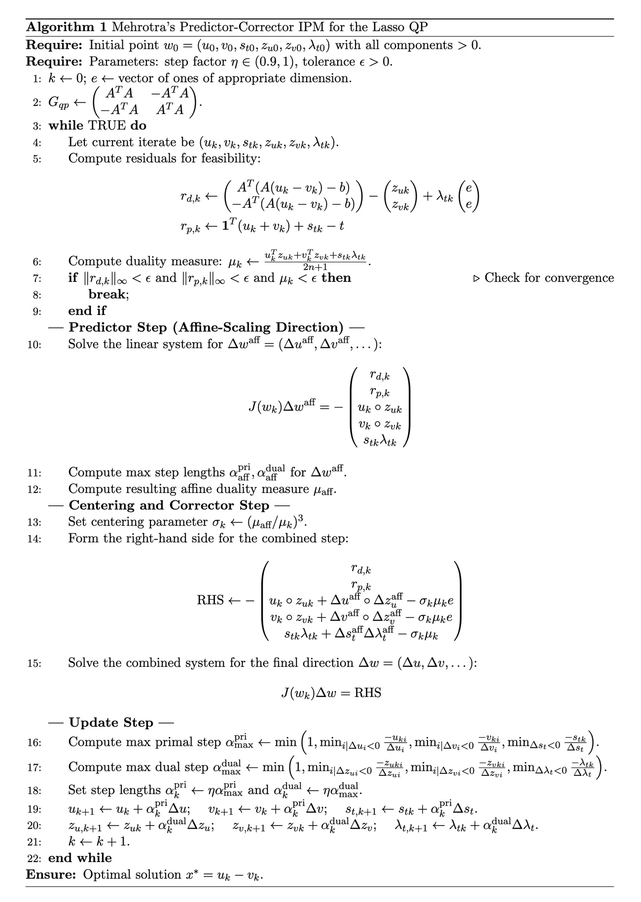
Each iteration of the solver follows five steps:
- Measure. Compute the primal and dual residuals and the duality measure μ.
- Predict. Solve a Newton system aimed straight at μ = 0, the affine-scaling direction.
- Correct. Set the centering parameter from the prediction, then add the second-order terms the linearization ignored.
- Update. Take separate primal and dual steps, cut at 99.5% of the distance to the boundary, so every variable stays strictly positive.
- Monitor. Stop when residuals and μ fall below the tolerance; record step sizes, regularization and numerical events.
The expensive part is the Newton system, of size (4n + 2) × (4n + 2). Eliminating the slack and dual directions reduces it to a symmetric positive definite system of size 2n × 2n:
The first block is constant and computed once, is diagonal and the last term is rank one: the trace of the budget constraint. Predictor and corrector share the same matrix and differ only in the right-hand side. This is the step, taken straight from lasso_ipm_solver.py:
# STEP 1: PREDICTOR (affine-scaling direction), a pure Newton step towards mu = 0rhs_comp_t_aff = -rc_tcorrection_from_t_aff = (rhs_comp_t_aff + lambda_t * r_p) / (s_t + eps)rhs_u_aff = -r_d1 - zu - correction_from_t_affrhs_v_aff = -r_d2 - zv - correction_from_t_affd_uv_aff = solve_linear_system_debug(np.concatenate([rhs_u_aff, rhs_v_aff]), "predictor")du_aff, dv_aff = d_uv_aff[:n], d_uv_aff[n:]ds_t_aff = -r_p - np.sum(du_aff + dv_aff)dzu_aff = (-rc_u - zu * du_aff) / (u + eps)dzv_aff = (-rc_v - zv * dv_aff) / (v + eps)dlambda_t_aff = (-rc_t - lambda_t * ds_t_aff) / (s_t + eps)# Centering parameter sigma (Mehrotra's heuristic)mu_aff = max(0, mu_aff_num / (2 * n + 1))sigma = (mu_aff / mu) ** 3 if mu > eps else 0.0# STEP 2: CORRECTOR, centering + second-order correctionrc_corr_u, rc_corr_v, rc_corr_t = du_aff * dzu_aff, dv_aff * dzv_aff, ds_t_aff * dlambda_t_affrhs_comp_t_corr = sigma * mu - rc_t - rc_corr_tcorrection_from_t_corr = (rhs_comp_t_corr + lambda_t * r_p) / (s_t + eps)rhs_u_corr = -r_d1 - (rc_u + rc_corr_u - sigma * mu) / (u + eps) - correction_from_t_corrrhs_v_corr = -r_d2 - (rc_v + rc_corr_v - sigma * mu) / (v + eps) - correction_from_t_corrd_uv = solve_linear_system_debug(np.concatenate([rhs_u_corr, rhs_v_corr]), "corrector")Show the full pseudocode Algorithm 1
Built not to break near the solution.
Close to the optimum the barrier terms explode and becomes ill-conditioned: a black-box call such as numpy.linalg.solve can stop on a singular matrix. The solver has two engines and a safety net:
- Cholesky factorization for small and medium problems: O(n³) per factorization, then two cheap triangular solves.
- Matrix-free conjugate gradient for high-dimensional problems, with a diagonal (Jacobi) preconditioner. is never formed: it is applied to vectors on the fly, which reduces the memory footprint.
- Adaptive regularization. A small is added to the system: it grows tenfold after a failed solve and decays by 1.5× after every successful iteration, so the original Newton system is perturbed only when it has to be.
# DIRECT METHOD (Cholesky, O(n^3)): M = G_qp + D_k + lambda/s * 11^T + delta * IM = G_qp + np.diag(diag_Dk_vec) + lambda_s_ratio * np.outer(e_2n, e_2n)current_reg = max(delta, base_reg_factor)M = M + current_reg * np.eye(2 * n)L, lower = cho_factor(M, lower=False, check_finite=False)solution = cho_solve((L, lower), rhs)# ITERATIVE METHOD (matrix-free CG): M is applied to vectors, never formeddef matvec(p): """Matrix-vector product for the KKT system.""" p_u, p_v = p[:n], p[n:] common_term = AtA_base @ (p_u - p_v) res_g = np.concatenate([common_term, -common_term]) res_d = diag_Dk_vec * p res_rank1 = (lambda_s_ratio * e_2n.dot(p)) * e_2n res_delta = current_reg * p return res_g + res_d + res_rank1 + res_deltaM_op = LinearOperator((2 * n, 2 * n), matvec=matvec)solution, info = cg(M_op, rhs, rtol=cg_rtol, maxiter=cg_maxiter, M=precond)# a failed solve multiplies delta by 10 and retries; every successful iteration lets it decay:delta = max(initial_delta, delta / 1.5)Same problem, fair comparison.
Libraries solve different versions of the Lasso, so a fair benchmark needs one problem for everyone. I fitted scikit-learn's penalized Lasso (α = 0.1), took the ℓ₁ norm of its solution as the budget t, and gave that same t to my solver and to CVXPY, with OSQP first and SCS as a fallback, both at tolerance 10⁻⁸. The two forms describe the same solution when , a scaling derived in the report.
| Dataset | Training | Test | Features | κ(AᵀA) |
|---|---|---|---|---|
| Diabetes | 331 | 111 | 10 | 4.18 × 10² |
| California Housing | 15,480 | 5,160 | 8 | 4.30 × 10¹ |
| IMDb | 111,324 | 37,108 | 19 | 3.59 × 10⁴ |
| Synthetic | 2,250 | 750 | 2,000 | 1.04 × 10³ |
Four datasets from small to high-dimensional: 75/25 split with fixed seeds, standardized on training statistics only. The synthetic set hides 9 informative features among 2,000.
Runtime, on a log scale
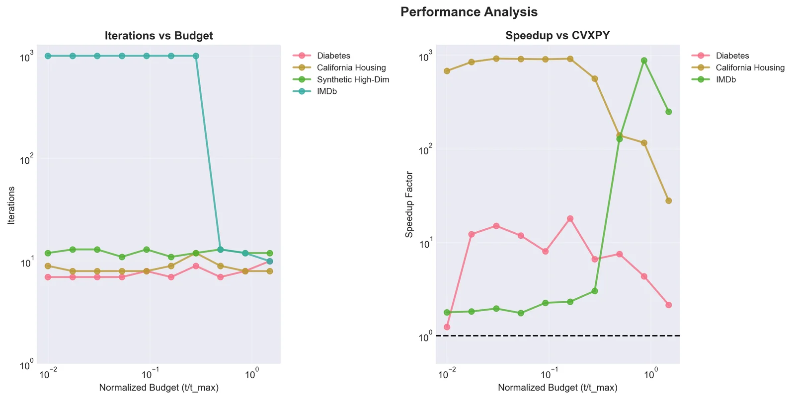
Wall-clock time for one solve at the common budget, from Table 5 of the report. OSQP solved Diabetes; on the other three datasets it failed or declared the problem infeasible, and SCS took over.
The same answer
| Dataset | My iterations | CVXPY iterations | ‖x − xCVXPY‖₂ | Active features |
|---|---|---|---|---|
| Diabetes | 7 | 1,425 | 1.08 × 10⁻⁸ | 4 / 10 |
| California Housing | 10 | 875 | 2.37 × 10⁻⁸ | 2 / 8 |
| IMDb | 200 | 1,975 | 3.48 × 10⁻⁸ | 3 / 19 |
| Synthetic | 12 | 4,925 | 1.16 × 10⁻⁷ | 8 / 2,000 |
Both solvers select exactly the same features, and test MSE, MAE and R² are identical on every dataset. On the synthetic set, all 9 true features are recovered along the regularization path, with no false positives at the best budget.
Few iterations, fast finish.
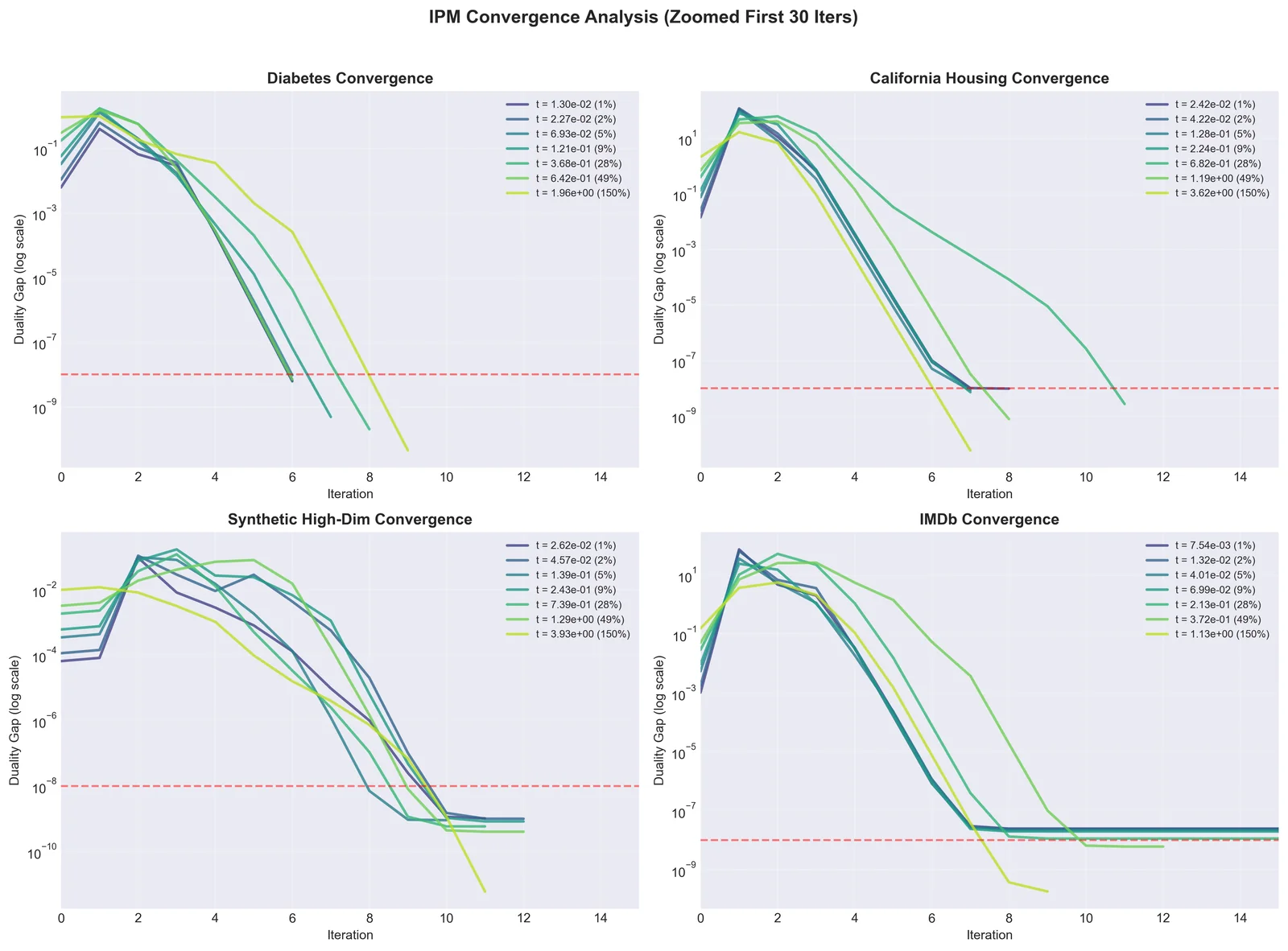
I swept ten budgets per dataset, from 1% to 150% of the unconstrained ℓ₁ norm. The duality gap follows the pattern the theory predicts: a centering phase, a transition, then a superlinear or quadratic finish. Of the 40 runs, 45% end quadratically and 37.5% superlinearly.
Every derivation is in the report.
Lagrangian and dual problem, convergence and complexity analysis, regularization paths and all the tables behind this page.